38 excel scatter graph data labels
Chart's Data Series in Excel - Easy Tutorial Select Data Source. To launch the Select Data Source dialog box, execute the following steps. 1. Select the chart. Right click, and then click Select Data. The Select Data Source dialog box appears. 2. You can find the three data series (Bears, Dolphins and Whales) on the left and the horizontal axis labels (Jan, Feb, Mar, Apr, May and Jun) on ... Prevent Overlapping Data Labels in Excel Charts - Peltier Tech 24-05-2021 · Overlapping Data Labels. Data labels are terribly tedious to apply to slope charts, since these labels have to be positioned to the left of the first point and to the right of the last point of each series. This means the labels have to be tediously selected one by one, even to apply “standard” alignments.
Excel: How to Create a Bubble Chart with Labels - Statology Step 3: Add Labels. To add labels to the bubble chart, click anywhere on the chart and then click the green plus "+" sign in the top right corner. Then click the arrow next to Data Labels and then click More Options in the dropdown menu: In the panel that appears on the right side of the screen, check the box next to Value From Cells within ...

Excel scatter graph data labels
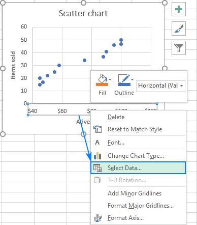
Add vertical line to Excel chart: scatter plot, bar and line graph 15-05-2019 · Right-click anywhere in your scatter chart and choose Select Data… in the pop-up menu.; In the Select Data Source dialogue window, click the Add button under Legend Entries (Series):; In the Edit Series dialog box, do the following: . In the Series name box, type a name for the vertical line series, say Average.; In the Series X value box, select the independentx-value … Labeling X-Y Scatter Plots (Microsoft Excel) - tips Just enter "Age" (including the quotation marks) for the Custom format for the cell. Then format the chart to display the label for X or Y value. When you do this, the X-axis values of the chart will probably all changed to whatever the format name is (i.e., Age). However, after formatting the X-axis to Number (with no digits after the decimal ... How to Add Labels to Scatterplot Points in Excel - Statology Step 3: Add Labels to Points. Next, click anywhere on the chart until a green plus (+) sign appears in the top right corner. Then click Data Labels, then click More Options…. In the Format Data Labels window that appears on the right of the screen, uncheck the box next to Y Value and check the box next to Value From Cells.
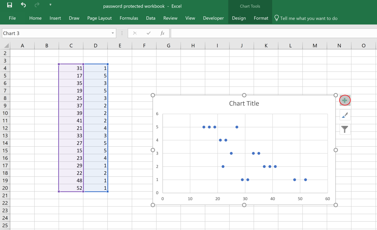
Excel scatter graph data labels. Present your data in a scatter chart or a line chart These data points may be distributed evenly or unevenly across the horizontal axis, depending on the data. The first data point to appear in the scatter chart represents both a y value of 137 (particulate) and an x value of 1.9 (daily rainfall). These numbers represent the values in cell A9 and B9 on the worksheet. Scatter Plots in Excel with Data Labels - LinkedIn Select "Chart Design" from the ribbon then "Add Chart Element" Then "Data Labels". We then need to Select again and choose "More Data Label Options" i.e. the last option in the menu. This will ... Find, label and highlight a certain data point in Excel scatter graph 10-10-2018 · But our scatter graph has quite a lot of points and the labels would only clutter it. So, we need to figure out a way to find, highlight and, optionally, label only a specific data point. Extract x and y values for the data point. As you know, in a scatter plot, the correlated variables are combined into a single data point. Scatter Graph - Overlapping Data Labels The use of unrepresentative data is very frustrating and can lead to long delays in reaching a solution. 2. Make sure that your desired solution is also shown (mock up the results manually). 3. Make sure that all confidential data is removed or replaced with dummy data first (e.g. names, addresses, E-mails, etc.). 4.
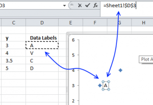
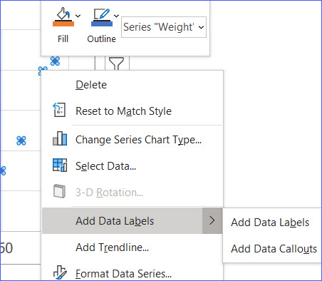
How to Change Excel Chart Data Labels to Custom Values? May 05, 2010 · Now, click on any data label. This will select “all” data labels. Now click once again. At this point excel will select only one data label. Go to Formula bar, press = and point to the cell where the data label for that chart data point is defined. Repeat the process for all other data labels, one after another. See the screencast. Add a DATA LABEL to ONE POINT on a chart in Excel All the data points will be highlighted. Click again on the single point that you want to add a data label to. Right-click and select ' Add data label '. This is the key step! Right-click again on the data point itself (not the label) and select ' Format data label '. You can now configure the label as required — select the content of ... Data label name appear on hover - Excel Help Forum Data label name appear on hover. I am trying to create an xy scatter plot with a lot of people in it, with a kpi for each axis, and each point has a name ( person 1 , person 2). I am trying to make the data labels appear only on hovering over by the mouse. i found this code online, (sorry cant remember who it was by , maybe peltier tech) , but ... Improve your X Y Scatter Chart with custom data labels - Get Digital Help Select the x y scatter chart. Press Alt+F8 to view a list of macros available. Select "AddDataLabels". Press with left mouse button on "Run" button. Select the custom data labels you want to assign to your chart. Make sure you select as many cells as there are data points in your chart. Press with left mouse button on OK button. Back to top
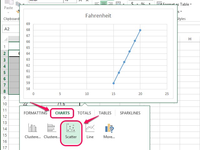
How to Make Charts and Graphs in Excel | Smartsheet 22-01-2018 · Because graphs and charts serve similar functions, Excel groups all graphs under the “chart” category. To create a graph in Excel, follow the steps below. Select Range to Create a Graph from Workbook Data. Highlight the cells that contain the data you want to use in your graph by clicking and dragging your mouse across the cells. Scatter plot excel with labels - dxhkpa.elnagh.com.pl Step 1: Select the data. Step 2: Go to Insert > Chart > Scatter Chart > Click on the first chart. Step 3: This will create the scatter diagram. Step 4: Add the axis titles, increase the size of the bubble and Change the chart title as we have discussed in the above example. Step 5: We can add a trend line to it. Change the format of data labels in a chart To get there, after adding your data labels, select the data label to format, and then click Chart Elements > Data Labels > More Options. To go to the appropriate area, click one of the four icons ( Fill & Line, Effects, Size & Properties ( Layout & Properties in Outlook or Word), or Label Options) shown here. Present your data in a scatter chart or a line chart 09-01-2007 · For example, when you use the following worksheet data to create a scatter chart and a line chart, you can see that the data is distributed differently. In a scatter chart, the daily rainfall values from column A are displayed as x values on the horizontal (x) axis, and the particulate values from column B are displayed as values on the vertical (y) axis.
Scatter Chart in Excel
How to add data labels from different column in an Excel chart? Right click the data series in the chart, and select Add Data Labels > Add Data Labels from the context menu to add data labels. 2. Click any data label to select all data labels, and then click the specified data label to select it only in the chart. 3.
Scatter Chart in Excel (Examples) | How To Create Scatter Chart in Excel?
Analytic Quick Tips - Building Data Labels Into an Excel Scatter Chart ... August 2014 - Building Data Labels Into an Excel Scatter Chart - Made Easy. Adding data labels to Excel scatter charts is notoriously difficult as there is no built-in ability in Excel to add data labels. While Microsoft does have a knowledge base page to add data labels, it is difficult to follow.
Excel: Scatter Charts are Versatile But Require a Different Workflow - Excel Articles
excel - How to label scatterplot points by name? - Stack Overflow select a label. When you first select, all labels for the series should get a box around them like the graph above. Select the individual label you are interested in editing. Only the label you have selected should have a box around it like the graph below. On the right hand side, as shown below, Select "TEXT OPTIONS".
Scatter Plot Template in Excel | Scatter Plot Worksheet
VBA Scatter Plot Hover Label | MrExcel Message Board Set ser = ActiveChart.SeriesCollection (1) chart_data = ser.Values chart_label = ser.XValues Set txtbox = ActiveSheet.Shapes ("hover") 'I suspect in the error statement is needed for this. If ElementID = xlSeries Then txtbox.Delete Sheet1.Range ("Ch_Series").Value = Arg1 Txt = Sheet1.Range ("CH_Text").Value
How to Make an XY Graph on Excel | Techwalla.com
How to Make a Scatter Plot in Excel (XY Chart)
How to Create a Scatter Plot in Excel - TurboFuture - Technology
Excel 2016 for Windows - Missing data label options for scatter chart Replied on October 12, 2017. You need to use the Add Chart Element tool: either use the + at top right corner of chart, or use Chart Tools (this tab shows up only when a chart is selected) | Design | Add Chart Element. By default this will display the y-values but the Format Labels dialog lets you pick a range. best wishes.

Scatter Chart in Excel
How to add text labels on Excel scatter chart axis - Data Cornering Stepps to add text labels on Excel scatter chart axis 1. Firstly it is not straightforward. Excel scatter chart does not group data by text. Create a numerical representation for each category like this. By visualizing both numerical columns, it works as suspected. The scatter chart groups data points. 2. Secondly, create two additional columns.
Find, label and highlight a certain data point in Excel scatter graph
How to Change Excel Chart Data Labels to Custom Values? 05-05-2010 · Now, click on any data label. This will select “all” data labels. Now click once again. At this point excel will select only one data label. Go to Formula bar, press = and point to the cell where the data label for that chart data point is defined. Repeat the process for all other data labels, one after another. See the screencast.
Improve your X Y Scatter Chart with custom data labels
3 Axis Graph Excel Method: Add a Third Y-Axis - EngineerExcel Scale the Data for an Excel Graph with 3 Variables. Excel allows us to add a second axis to a scatter chart and we’ll use this for velocity and acceleration. ... Axis labels were created by right-clicking on the series and selecting “Add Data Labels”. By …
Improve your X Y Scatter Chart with custom data labels
The Problem With Labelling the Data Points in an Excel Scatter Chart Labelling the data points in an Excel chart is a useful way to see precise data about the values of the underlying data alongside the graph itself. In a column chart, for instance, you might show the value of the data point at the top of a column. A useful addition to a column chart is a set of data labels showing the value of each column.
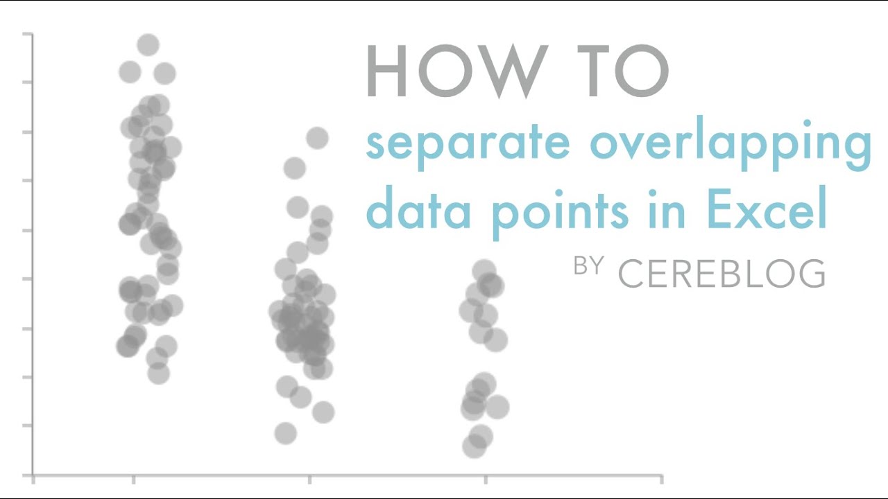
How to separate overlapping data points in Excel - YouTube
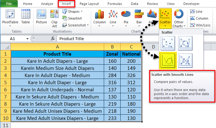
How To Create Scatter Chart in Excel? - EDUCBA To apply the scatter chart by using the above figure, follow the below-mentioned steps as follows. Step 1 - First, select the X and Y columns as shown below. Step 2 - Go to the Insert menu and select the Scatter Chart. Step 3 - Click on the down arrow so that we will get the list of scatter chart list which is shown below.

I am working on an excel scatter graph. I have about 80 rows of data and am using filters to ...
Creating Scatter Plot with Marker Labels - Microsoft Community Right click any data point and click 'Add data labels and Excel will pick one of the columns you used to create the chart. Right click one of these data labels and click 'Format data labels' and in the context menu that pops up select 'Value from cells' and select the column of names and click OK.

Line Chart in Excel - Easy Excel Tutorial
How to display text labels in the X-axis of scatter chart in Excel? Display text labels in X-axis of scatter chart Actually, there is no way that can display text labels in the X-axis of scatter chart in Excel, but we can create a line chart and make it look like a scatter chart. 1. Select the data you use, and click Insert > Insert Line & Area Chart > Line with Markers to select a line chart. See screenshot: 2.
How to Make a Scatter Chart - ExcelNotes
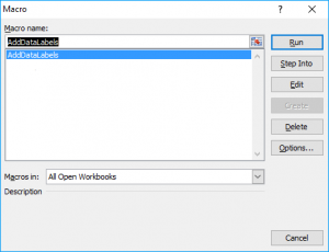
Create an X Y Scatter Chart with Data Labels - YouTube How to create an X Y Scatter Chart with Data Label. There isn't a function to do it explicitly in Excel, but it can be done with a macro. The Microsoft Kno...
Create Excel Scatter Chart in C#
Excel scatter chart using text name - Access-Excel.Tips Solution - Excel scatter chart using text name. To group Grade text (ordinal data), prepare two tables: 1) Data source table. 2) a mapping table indicating the desired order in X-axis. In Data Source table, vlookup up "Order" from "Mapping Table", we are going to use this Order value as x-axis value instead of using Grade.
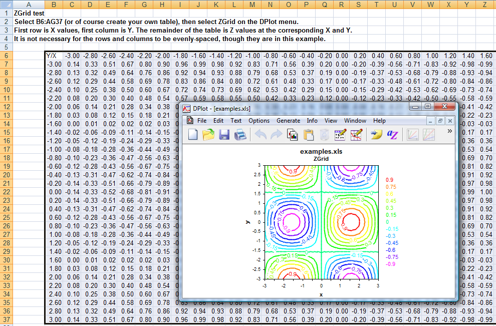
Getting Started > Getting Started with XYZ Surface Plots > Getting Started with XYZ Surface ...
3 Axis Graph Excel Method: Add a Third Y-Axis - EngineerExcel By default, Excel adds the y-values of the data series. In this case, these were the scaled values, which wouldn’t have been accurate labels for the axis (they would have corresponded directly to the secondary axis). However, in Excel 2013 and later, you can choose a range for the data labels. For this chart, that is the array of unscaled ...

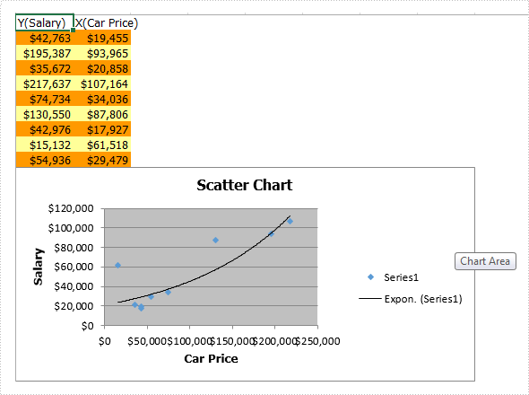
Everyday Statistics for Programmers: Nonlinear Regression
Find, label and highlight a certain data point in Excel scatter graph Oct 10, 2018 · But our scatter graph has quite a lot of points and the labels would only clutter it. So, we need to figure out a way to find, highlight and, optionally, label only a specific data point. Extract x and y values for the data point. As you know, in a scatter plot, the correlated variables are combined into a single data point.

Xyz graf excel | there are several different equations you need in order
Add Custom Labels to x-y Scatter plot in Excel Step 1: Select the Data, INSERT -> Recommended Charts -> Scatter chart (3 rd chart will be scatter chart) Let the plotted scatter chart be. Step 2: Click the + symbol and add data labels by clicking it as shown below. Step 3: Now we need to add the flavor names to the label. Now right click on the label and click format data labels.
Post a Comment for "38 excel scatter graph data labels"